Machine Learning Projects
The three machine learning projects I completed during my master’s at Imperial are summarised:
1. Rock Characterisation
Summary: For my Machine Learning class project, I created a lithology estimator using Python. I used scikit-learn, pandas, and numpy for implementation and integrated data preprocessing into streamlined pipelines. I developed custom transformation functions and encapsulated the entire workflow within a Python class. This modular approach facilitated model selection and its future use in different test cases. After hyperparameter tuning, I achieved an R2 score of 0.89 with logistic regression, whereas the dummy model only had an R2 score of 0.20.
Problem: Ocean floor is drilled to understand what type of rock present. Since recovering the rock core is expensive, an AI model that predicts lithology (type of rock) from the log data needs to be created.
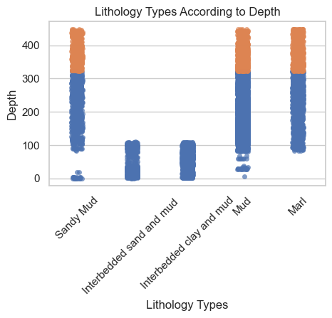
A spatial train test split is preferred because we are trying to estimate the deepest locations in the subsurface. The test set is indicated by orange, while the training and validation set is indicated by blue:
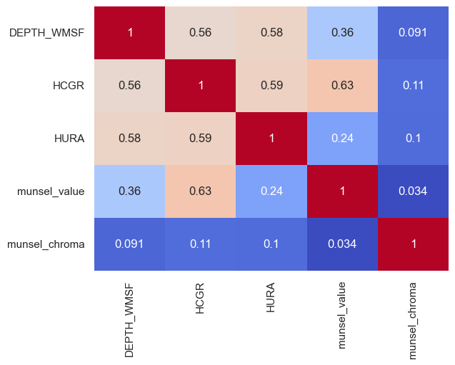
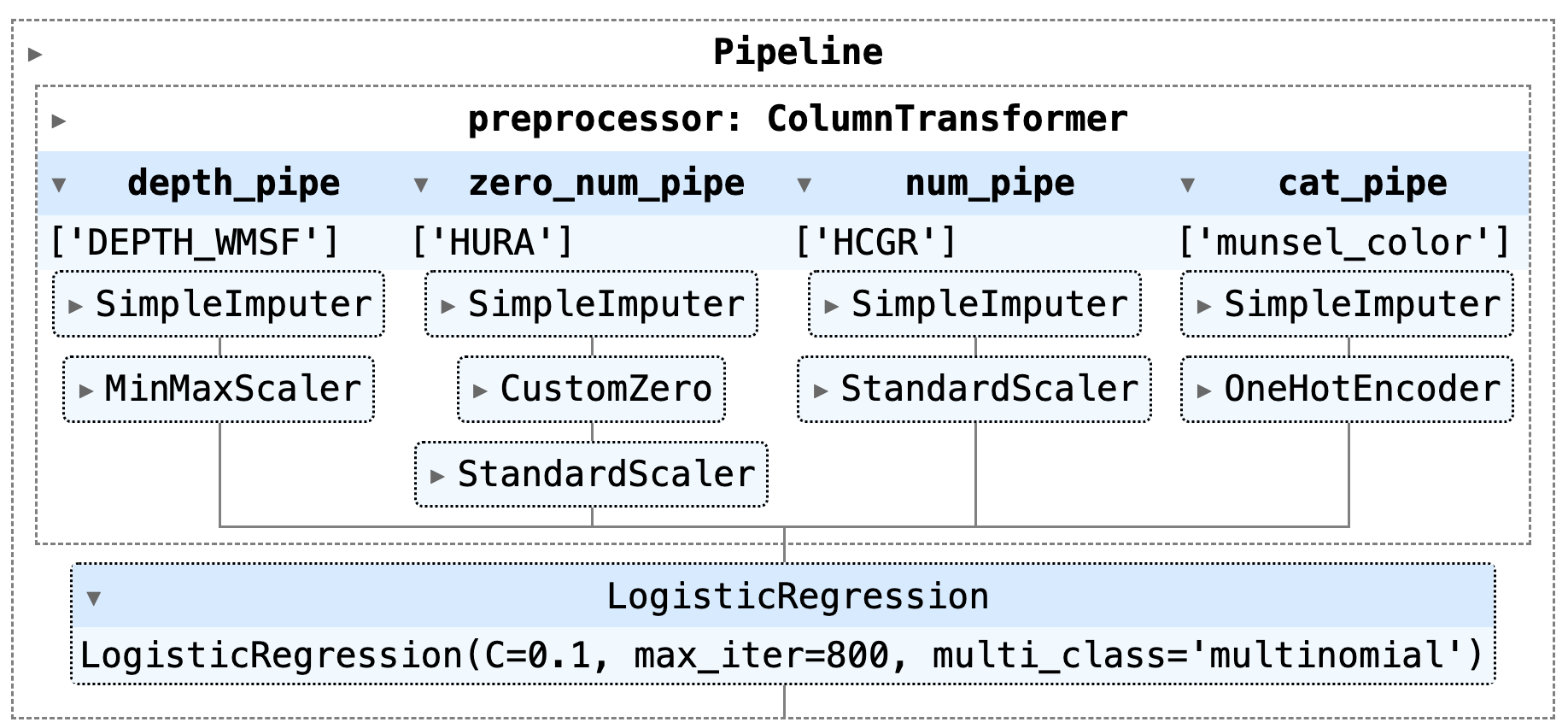
Exploratory data analysis is carried out for feature selection. In the end, I continued with the following features, including depth DEPTH_WMSF, total gamma ray HCGR, uranium HURA, and munsel color:
Each feature requires different preprocessing steps, such as encoding and scaling, based on its properties, such as being categorical or having a skewed distribution. These preprocessing steps are encapsulated in pipelines shown below:
2. Medical Image Generation
I did this as an individual project as part of my Deep Learning class using PyTorch. Medical datasets are often limited due to the rarity of certain conditions or privacy concerns. Thus, I designed a Variational Autoencoder (VAE) to generate synthetic x-ray images of hands using a dataset of 8000 X-ray scans.
I specifically chose to use a VAE because of its explainability and specific nice features, such as the reparametrization trick and customizing the loss function with Kullback-Leibler (KL) Divergence.
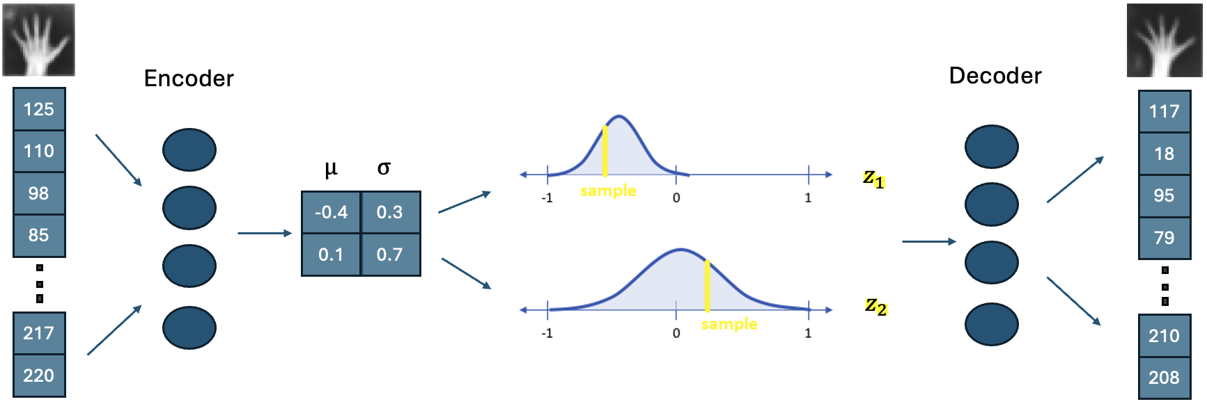
The 32x32 grayscale hand images are compressed into a two-dimensional latent space. The values in this space are treated as statistical parameters of a Gaussian distribution. New values are generated by randomly sampling from these distributions and then inputted into the decoder to create a new image. This random sampling acts as a regulariser and helps prevent overfitting.
Because we need to take the derivative of each step during backpropagation, and sampling from a distribution is not differentiable, we apply the reparametrization trick as follows:
- $\epsilon$ is sampled from $N(0,1)$
- $z = \mu + \sigma \epsilon$
- $\frac{dz}{d\mu}, \frac{dz}{d\sigma}$ is possible
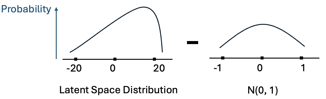
The loss function of a VAE consists of the sum of two components: the reconstruction loss and the KL divergence. The KL divergence measures the similarity between two distributions. In our case, it is the difference between the latent space distribution and the Gaussian distribution. This helps us create a more uniform and smooth latent space, with values centered around 0.
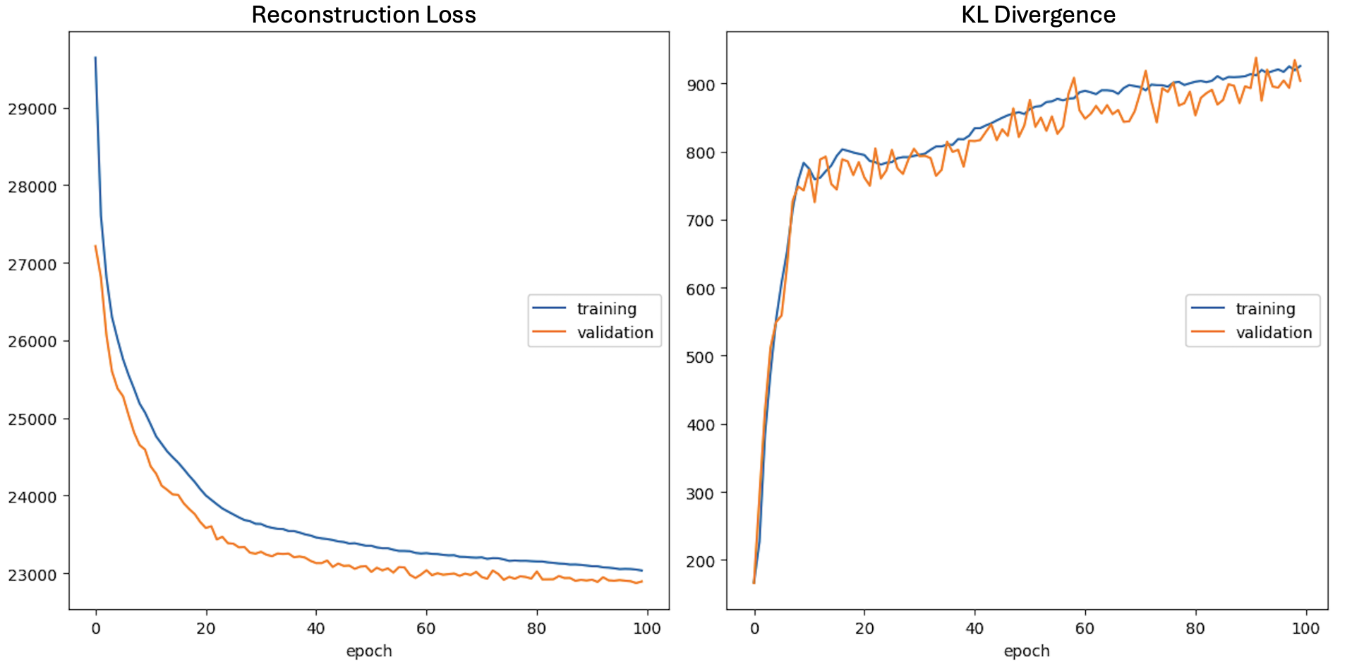
Model is trained with 8000 hand images. The evolution of the Reconstruction Loss and KL Divergence Loss during the training process can be found below:
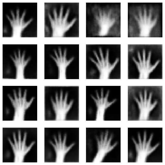
A grid of randomly generated hand images can be found below:
3. Storm Prediction
This was a group project with 6 students. I was responsible for leading the team, creating common data handling classes and packaging them, managing the project and version control of team members’ contributions on GitHub, creating the image generation LSTM architecture based on differences of consecutive images, and integrating three different machine learning models to predict future wind speeds.
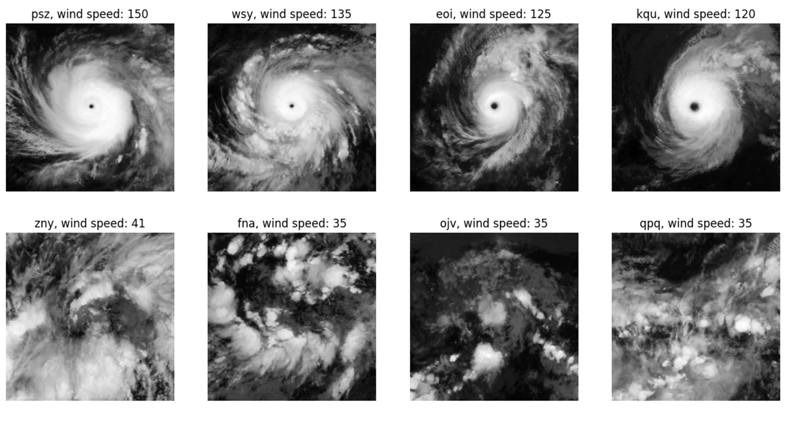
The first model was developed by my team mates which estimated the maximum wind speed of a storm at a specific time by analyzing a snapshot satellite image of the storm. Since storms have specific shapes when they gain speed, it was possible for a CNN to understand the wind speed from patterns in the images.
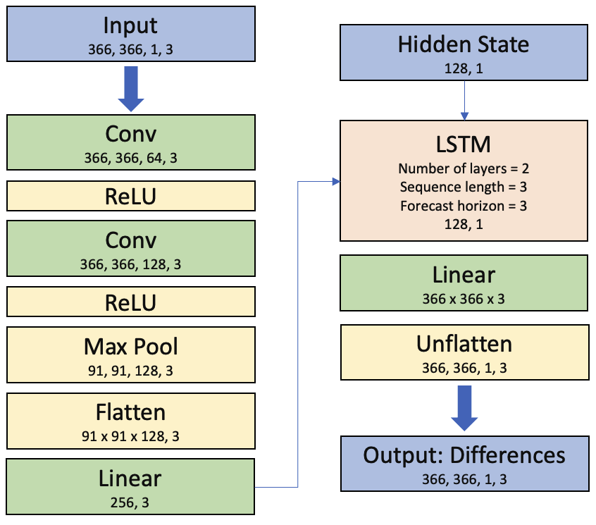
The second model was developed by me. It is a convolutional LSTM that learns the differences between consecutive images. First, the high-dimensional input is reduced to a size that the LSTM can handle. The last hidden state, which contains information about the entire sequence, is then fed into a linear layer where it is shaped into our desired output format. The architecture can be seen below:
Our objective was to capture the turning motion in consecutive images, a goal we successfully achieved, as demonstrated in the GIF below. Notably, the last three images in the GIF, which are brighter, were created by our model. You may observe some overall noise and increased brightness in the generated images, which could be reduced through post-processing in a future study.
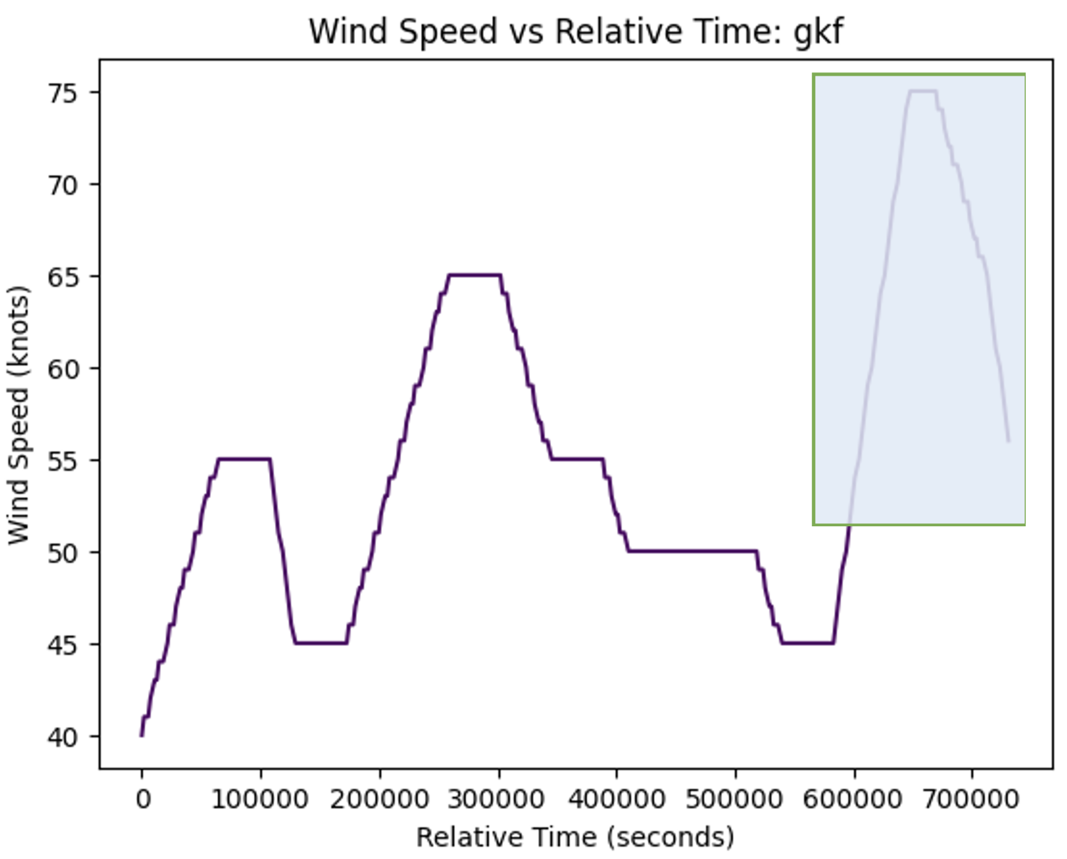
The last model is a direct LSTM forecast that uses only the time series wind speed data not the images. Data from 30 different real-world storms are used to train this LSTM model.