
Full Waveform Inversion
This individual project was part of my Optimization and Inversion class at Imperial College London.
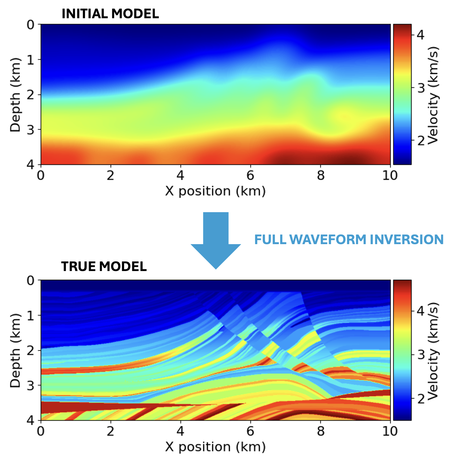
I set up the acquisition geometry to generate synthetic shot recordings, implemented the full waveform inversion (FWI) algorithm using the Armijo rule to determine the step size. The implementation was done in Python, utilising the Devito package. The well-known Marmousi dataset, which represents a geological model from Angola, was used for testing. The initial model was a smoothed version of the true dataset to provide a reasonable starting point for inversion.
Acquisition Geometry
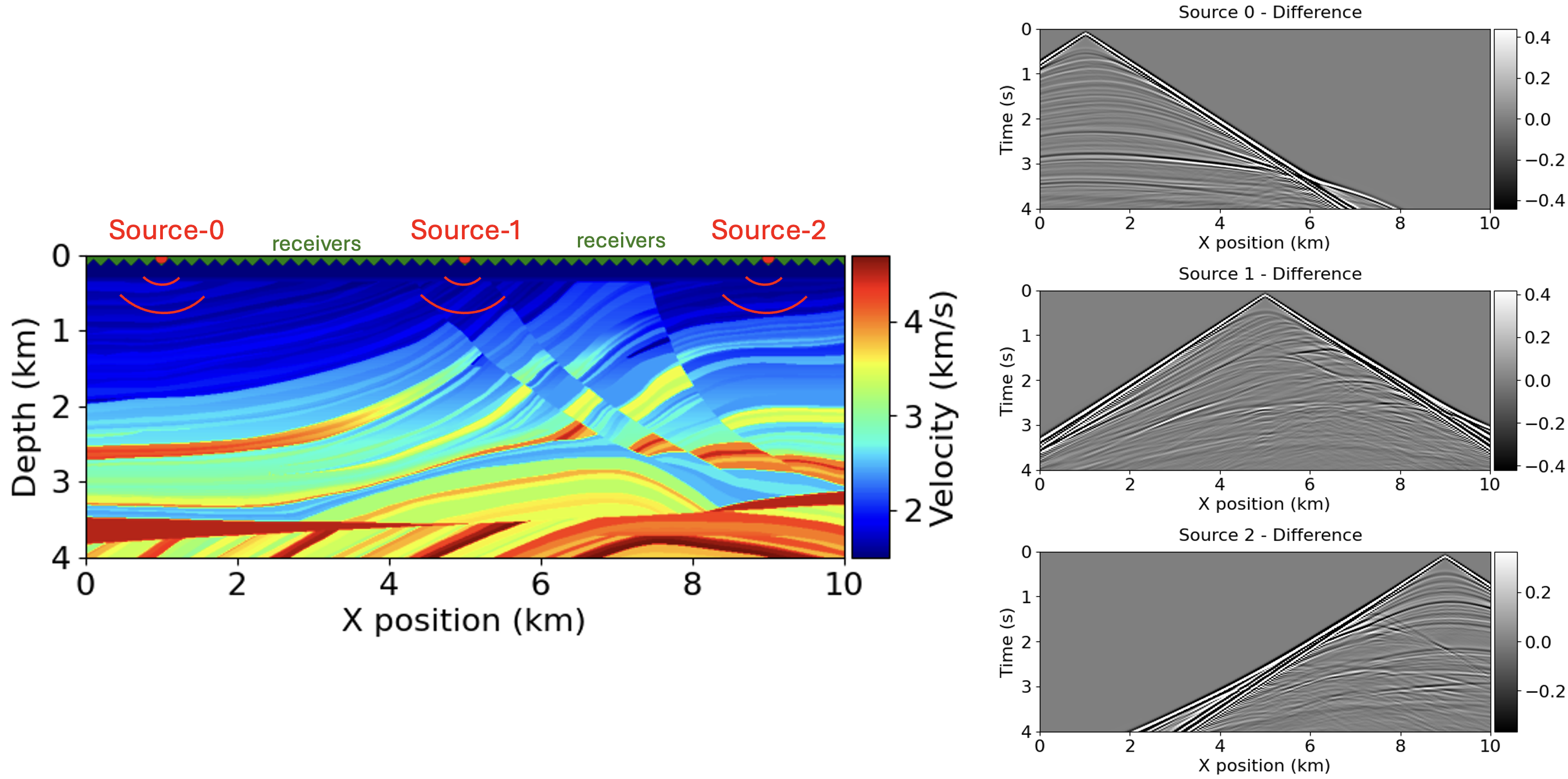
The sources and receivers were placed 20m below ground to ensure they are within the subsurface, with sources spanning from 1km to 9km at equal intervals to avoid boundary reflections.
Source Wavelet
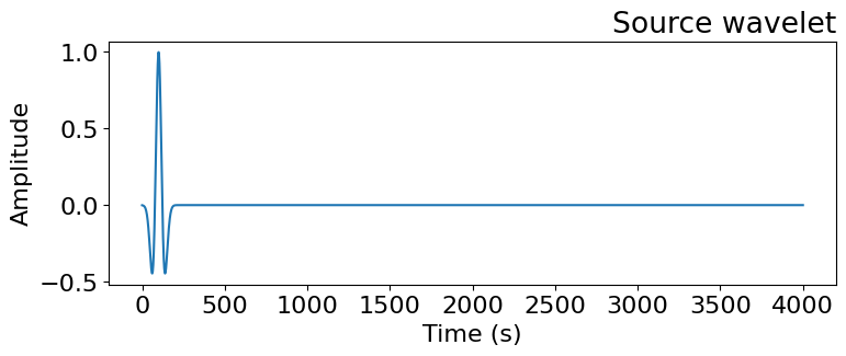
I used a Ricker wavelet with a peak frequency of 10Hz, balancing resolution and wave penetration depth, and set the simulation end time to 4 seconds to capture meaningful wave reflections while avoiding redundant late arrivals.
Algorithm
We will update the velocity profile of the grid in every iteration. The model update scheme is as follows:
$ m_{n+1} = m_n + \alpha \mathbf{p} $
- $m$: model parameters meaning velocity profile of the subsurface
- $\alpha$: update distance of each iteration
- $\mathbf{p}$: update direction
- A suitable choice for update direction is $\mathbf{p} = - \nabla_m f/ $.
- $\nabla_mf$ gives us the steepest direction thus we reverse it with ‘$-$’ sign. Then we divide the gradient by its norm as we want our direction to be unit length.
- Note that, there are improved direction selection algorithms like conjugate gradient method which selects the direction conjugate to the previous residual.
As we know our update direction, all we need to do is find $\alpha$. We will use Armijo rule which can be represented by the following:
\[f(\mathbf{m} + \alpha \mathbf{p}) - f(\mathbf{m}) \leq \beta\alpha\nabla f(\mathbf{m})^T\mathbf{p},\]Finding the update direction:
Forward model: major computation due to solving the matrix equation, synthetic data is simultaneously created.
\[A(\mathbf{m})\mathbf{u} = \mathbf{d}_{\text{syn}}\]Forming residuals: little computation.
\[\mathbf{r} = p\mathbf{u} - \mathbf{d}_{\text{obs}}\]Backpropagating the residuals: major computation. Again, computation is due to solving wave equation for adjoint wavefield $v$.
\[A^T(\mathbf{m})\mathbf{v} = \mathbf{p}^T\mathbf{r}\]- Note that $\mathbf{p}$ is a scaling matrix here to ensure compatibility.
Compute gradient: The gradient of the objective function is found by cross-correlating the forward wavefield ($\mathbf{u}$) and the adjoint wavefield ($\mathbf{v}$)